Warning: include(/data/htdocs/hebergementweb/sites/imagemed.univ-rennes1.fr/en/nav.html): failed to open stream: No such file or directory in /data/htdocs/hebergementweb/sites/imagemed.univ-rennes1.fr/template.php on line 144
Warning: include(): Failed opening '/data/htdocs/hebergementweb/sites/imagemed.univ-rennes1.fr/en/nav.html' for inclusion (include_path='.:/usr/share/pear:/data/htdocs/hebergementweb/php-include') in /data/htdocs/hebergementweb/sites/imagemed.univ-rennes1.fr/template.php on line 144
Principle of joint quantification of iron and hepatic fat by MRI

The hepatic iron concentration (CHF) can be estimated by calculating T2* or the signal intensity ratio between the liver is the paravertebral muscles (SIR method).
The evaluation of the fat fraction (FF) can be done via imaging phase by comparing the liver signal on the images in phase and in opposed phase. A joint estimation is necessary because each overload can influence the quantification of the other overload
Quantification of iron
In histology, in case of iron overload, a Perls's staining highlights blue elements corresponding to iron deposits. Liver Iron Concentration (LIC) has been determined for a long time by the biochemical analysis of the biopsy fragment and is expressed as either mg/g liver dry weight with a maximum normal value of 2 mg/g, ie in μmol/g with a maximum normal value of 36μmol/g because there is a relationship of 1 to 18 between mg and μmol. This method causes the destruction of the biopsy block. It is less and less performed and replaced by MRI
MRI is a technique sensitive to the existence of iron within tissues. Indeed, iron is a paramagnetic substance that becomes superparamagnetic (with a strong decrease of the T2*), when several atoms are grouped as it is observed within the hemosiderin. In the context of an iron overload, its presence in the liver therefore leads to a significant drop in the signal by collapse of the T2* relaxation time. This hyposignal is proportional to the importance of the overload. It is easier to detect using gradient echo sequences because they are rephased by magnetic field gradients and not by 180 ° radio frequency waves. This makes them more sensitive to the local heterogeneity of the magnetic field. The signal drop is then specific when using in-phase TEs to suppress the influence of the fat.
The precise quantification of the iron overload can be done by two methods which have been validated in the literature. They each have their advantages and disadvantages. They have long opposed them but in our opinion they are complementary.
The liver to muscle ratio or SIR (signal intensity ratio)
This is the method that we initially proposed ( Lancet 2004) and which was also implemented by Alustiza ( Radiology 2004) with a formula based on 2 echoes. Rose ( Eur J Haematol 2006) proposed to add a sequence with a shorter TE, in opposition of phase, for quantifying heavy overloads.
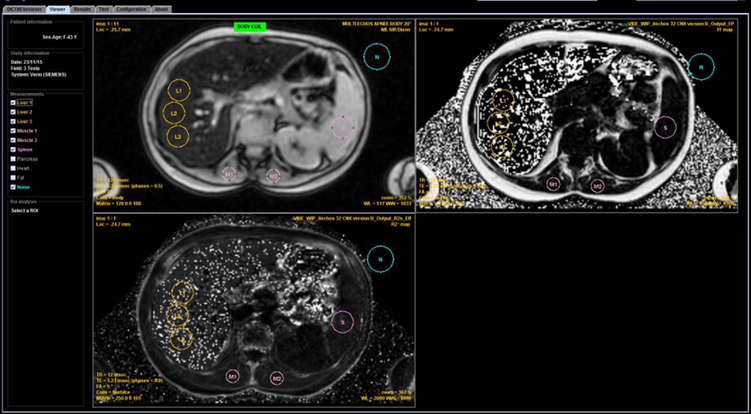
It is simple to implement and has long been the most used method because it does not require any technical constraint. It compensates for the absence of calibrated value in MRI by a relative value, by quantitatively comparing the signal of the liver with that of the paravertebral muscles. This makes it necessary to use the integrated body antenna in the tunnel wall, without any intervention of the surface antennas, in particular those integrated in the bed in order to avoid any signal gradient between the surface and the depth. Then, a strict acquisition protocol based on apnea gradient echo sequences with a TR of 120 ms, a 20° flip angle and TE in phase,to limit the influence of the fat, must be applied. The values of the TEs are therefore dependent on the magnetic field. A first very short echo, in opposition of phase, can be added to quantify the very strong overloads but it should be taken into account only in case of strong overload with a regular decay of the signal on the successive echoes and not the use in case of signal undulate in connection with steatosis
| Sequence | TR (ms) | FA (°) | TE (ms) | |
|---|---|---|---|---|
| 1.5T | 3T | |||
| Out | 120 | 20 | 2.4 | 1.2 |
| DP | 120 | 20 | 4.8 | 2.4 |
| T2 | 120 | 20 | 9.6 | 4.8 |
| T2 | 120 | 20 | 14 | 9.6 |
These mono-echo sequences can be reduced to only one by acquiring a multi-echo sequence comprising multiple TEs of 1.2 or 2.4 ms to 1, 5T or 1.2 ms to 3T. However, care must be taken to obtain at least all the in-phase echo time required for the calculation.
In a normal patient, the liver signal is greater than that of the muscle on short TEs and only slightly falls below that of the muscle on the longest TEs
In case of moderate iron overload, the signal of the liver is close to that of the muscle on the shortest TE and falls rapidly below that of the muscle with elongation. TE
In case of significant iron overload, the liver signal is already lower than that of the muscle in the shortest TE and collapses rapidly with TE elongation.
If the liver signal intensity on the shortest, opposed-phase, TE is lower th signal of the following in-phase TE it reflects the presence of associated fat infiltration and this opposed-phase TE cannot be use for quantification.
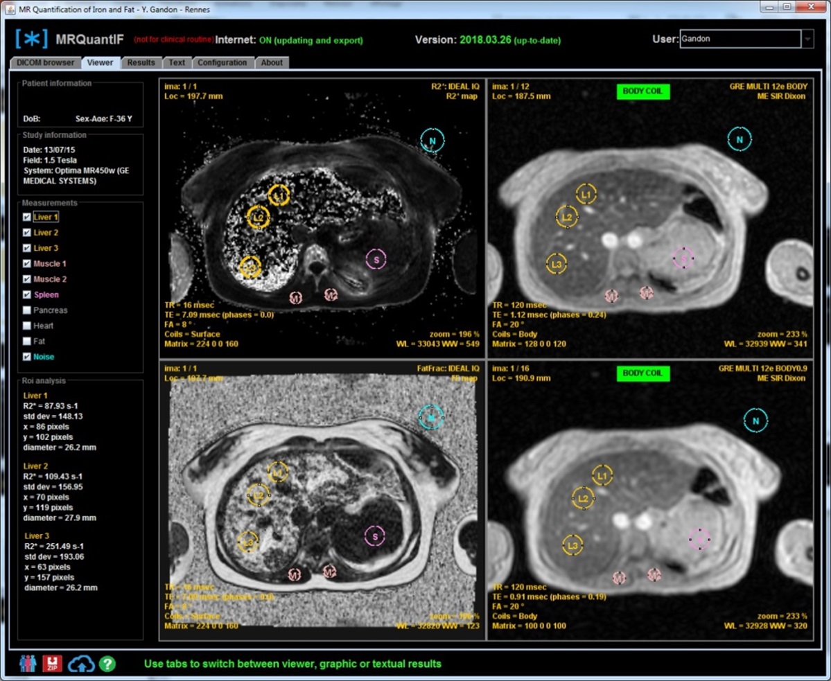
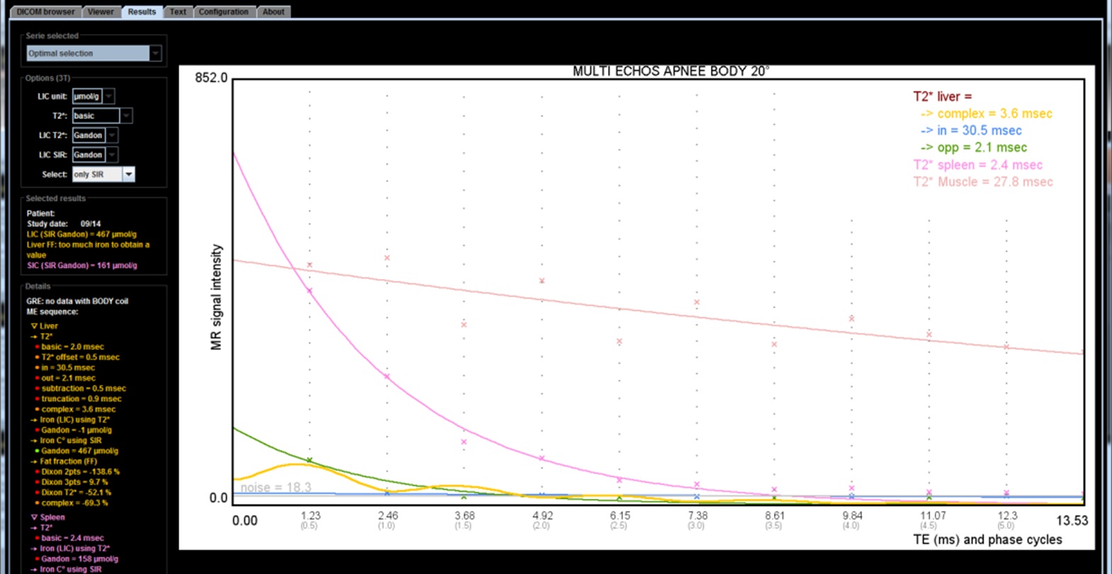
To obtain precise quantification, several measurements must be made by an ROI on the most homogeneous areas of the liver and paraspinal muscles. The measurements can be done on a DICOM workstation and retranscribed in the in-line module. But this formula overestimate the LIC and many potentially serious errors can be made if other coils than the tunnel antenna have been selected. This is why we recommended to migrate progressively to the DICOM MRQuantif software which controls the acquisition parameters.
At 1.5 Tesla
Two calculation SIR methods have been published: our method "Gandon" corresponding to the online calculation, which, in agreement with the publication of Castiella, certainly overestimates the moderate overloads, and "Alustiza" which gives lower values but more consistent with the values obtained by T2*. In order to make the values more comparable, the MRQuantif software now propose to use the Alustiza algorithm by default. As our knowledge evolves, we will adapt the MRQuantif tool to provide you with the most robust value in all circumstances. However we will see that it is probably better to use the calculation of R2* (1 / T2*) for low or moderate overloads and to switch to the SIR method for heavy overloads.
| Ref | Patients | With biopsies | LIC range (µmolg/g) |
Sequence | Matrix | TR (ms) |
FA (°) |
TE-min (ms) |
N TEs | TE-max (ms) |
Method | Correlation (R) | ||
|---|---|---|---|---|---|---|---|---|---|---|---|---|---|---|
| Gandon The Lancet 2004 |
113 patients + 61 controls |
174: with cirhosis (n=39), with steatosis (n=31) |
0-709 | GRE mono echo |
256×128 | 120 | 20 | 4 | 4 | 21 | on-line calculator | 0.87-0.92 | ||
| Alustiza Radiology 2004 |
44 patients + 68 controls |
112 | 0-390 | GRE mono echo |
256×128 | 120 | 20 | 4 | 3 | 21 | formula | 0.94 | ||
| Rose Eur J Haematol 2006 |
25 patients + 2 controls |
27 | 25-972 | GRE mono echo |
256×128 | 120 | 20 | 1.8 | 5 | 21 | formula for high overload using 1.8 ms TE |
0.85 | ||
| Castiella Eur Radiol 2011 |
64 patients (20 new) + 107 controls (39 new) |
112 published(Alustiza) +59 new |
0-390 | GRE mono echo |
256×128 | 120 | 20 | 4 | 3 | 21 | 31 patients at 1T, TE 9 ms missing |
0.86 | ||
| Total of 372 biopsies | ||||||||||||||
At 3 Tesla
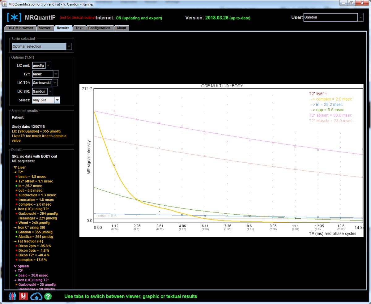
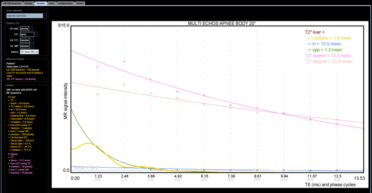
There is only our algorithm published in 2017 in Abdominal radiology. It was perfectly calibrated in confrontation with biopsies. It gives a similar result to the T2* method by applying our conversion formula ( European radiology 2017). At this magnetic field the T2* is twice as short and is reduced very quickly in case of iron overload. We will see that it can become difficult to obtain TEs short enough to calculate a collapsed T2*. In these circumstances, the SIR method is preferable and the software chooses the optimal method according to the result.
| Ref | Patients | With biopsies | LIC range (µmolg/g) |
Sequence | Matrix | TR (ms) |
FA (°) |
TE-min (ms) |
N TEs | TE-max (ms) |
Method | Correlation (R) | ||
|---|---|---|---|---|---|---|---|---|---|---|---|---|---|---|
| Paisant Abd Radiol 2017 |
105 patients | 105: hemochromatosis (n=31) DIOS (n=22) others (n=3) controls (n=49) |
0-630 | GRE mono echo |
106×128 | 120 | 20 | 1.2 | 5 | 14 | on-line calculator | 0.96 | ||
| Total of 105 biopsies | ||||||||||||||
The calculation of T2* or R2* (= 1 / T2*) and its conversion to hepatic iron concentration
T2* is the exponential decay parameter of the signal observed in gradient echo. It decreases rapidly in the presence of iron in the crystalline form, as in the case of hemosiderin which is the form of storage of hepatic iron. T2* can be calculated from the signal measured on a sequence with several echoes by an optimization method ( Levenberg-Marquardt or simplex) using the decay formula of the signal :
When the TE is equal to T2* there has been a decrease of about 2/3 of the signal. It will therefore be necessary to have measurements with TE shorter than the T2* assumed to obtain a correct estimate of T2*. So if the T2* is close to 1 ms and the first measured TE is also 1 ms the accuracy is not as good as if you can get a first TE at 0.5 ms. There could be a significant error of estimation if the T2* is shorter than the first TE with a value of T2* which can even go up quickly because the estimation of the starting signal can become completely erroneous. This explains the difficulties observed at 3T in case of heavy overloads because the iron effect and then the decrease of the T2* is proportional to the magnetic field.
In practice there are several ways to calculate T2*. They are available in the MRQuantif software and can be selected from a drop-down menu in the calculation options:
- T2* basic: this calculation is taking all the measurements of the liver signal, without taking into account the phase. This formula ignores any background noise measured or calculated. It is therefore understandable that the measurement may be disturbed by the presence of fat or distorted in the event of significant collapse of the signal.
- T2* offset: it's the same thing but considering that there is an offset corresponding to the background noise. This unknown is calculated by the estimate. In practice, the offset value obtained is sometimes false and far from the measured value of the background noise. The value is also distorted when there is a strong steatosis because the signal undulates between the phase and the phase opposition.
- T2* in: this is similar to the T2* basic calculation but taking only the liver signal measurements for TEs close to the in-phase values.
- T2* out: this is similar to the T2* basic calculation but taking only the liver signal measurements for TEs close to the opposed-phase values.
- T2* subtraction: it's the same as the T2* basic, but subtracting the background signal from the liver signal (calculated by offset or measured). This method often leads to a reduction in T2*.
- T2* truncation: it's the same as the T2* basic but stopping to take into account the values of the hepatic signal from the first measurement which is equal or inferior at background noise. It is certainly the most logical method but it can also be faulted if the signal is collapsed.
- T2* extrapolation: it's the same as the T2* truncation but adding fictitious values adapted to the shape of the curve (personal idea not yet evaluated).
- T2* complex: the calculation is done by integrating in the equation the percentage of fat and its influence on the signal. This is the best theoretical method and the only one actually applicable in case of steatosis. But conversely the introduction of a new unknown makes him lose some strength. In case of very high iron overload, it can lead to aberrant results with a slightly modified R2* and a very high fat overload when in fact there is no steatosis.
The T2* is the absolute numerical value that directly appreciates the presence of iron. It took many years to come to the fore because it ideally imposes a multi-echo sequence . The first major publication that established this method was done by Wood ( Blood 2005 ) who proposed to perform repeated mono-echo sequences without re-calibration. The shortest TE used was 0.8ms. At taht time to obtain this value it had to reduce the matrix to 64x64 pixels. Today all the main systems propose a 2D or 3D multi-echo sequence but it is not easy to get the first TE down below 1 ms with these multiecho sequences.
At 1.5 Tesla
Several studies compared the results of the calculation of R2* with that of CHF obtained by biopsy. The main ones are:
| Ref | Patients | With biopsies | LIC range (mg/g) |
Sequence | Matrix | TR (ms) |
FA (°) |
TE-min (ms) |
delta-TE (ms) |
N TEs | TE-max (ms) |
Comment | Method | Correlation (R) |
|---|---|---|---|---|---|---|---|---|---|---|---|---|---|---|
| Anderson Eur Heart J 2001 |
27 patients | 27 (29 biopsies): β-thalassemia | 1-26 | GRE mono echo |
96×128 | 200 | 20 | 2.2 | 2.56 | 8 | 20.1 | offset | 0.68 (fibrosis) 0.93 (others) |
|
| Wood Blood 2005 |
102 patients + 13 controls |
22: thalassemia major (n=9), sickle cell disease (n=10), thalassemia intermedia (n=2), Blackfan-Diamond syndrome (n=1) |
1.3-32.9 et 57.8 |
GRE mono echo |
64x64 | 25 | 20 | 0.8 | 0.25 | 16 | 4.8 | Controls: R2* = 39 s-1 T2* = 25 ms. |
offset | 0.97 |
| Hankins Blood 2009 |
43 patients | 43: sickle cell disease (n=32), thalassemia major (n=6), bone marrow failure (n=5) |
0.6-27.6 NB: 2 <2mg/g |
GRE multi echoes |
? | ? | ? | 1.1 | 0.8 | 20 | 17,3 | truncated | 0.97 | |
| Garbowski J Cardiovasc Magn Reson 2014 |
121 patients 31 controls |
25 (50 biopsies): βthalassemia (n=20), Blackfan-Diamond syndrome (n=1), congenital sideroblastic anemia (n=2), pyruvate kinase deficiency (n=1) |
1.7-42.3 NB: 1 <2mg/g |
GRE multi echoes |
? | ? | ? | 1.1 | 0.8 | 20 | 17,3 | Controls: R2* = 37 s-1 T2* = 27 ms. |
truncated | 0.94 |
| Henninger RöFo 2015 |
17 patients | 17: hemochromatosis (n=10), DIOS (n=2), aceruloplasminemia (n=2), congenital sideroblastic anemia (n=1), spur cell aenemia (n=1) |
0.92-11.65 NB: 4 <2mg/g |
GRE multi echoes |
128x128 | 200 | 20 | 0.99 | 1.41 | 12 | 16.5 | fat suppression | truncated | 0.92 |
| Total of 161 biopsies | ||||||||||||||
Looking at the main curves correlating R2* and LIC expressed in mg/g we see that the quantification becomes uncertain beyond 30 mg/g to 1.5T, and even less in the Garbowski study:
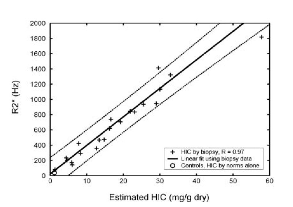
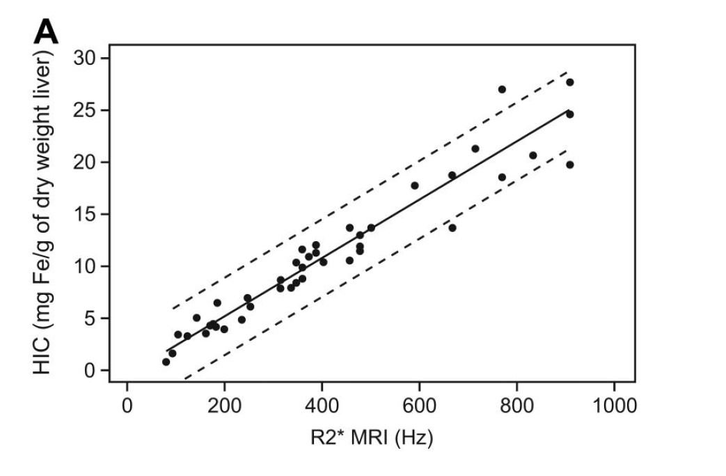
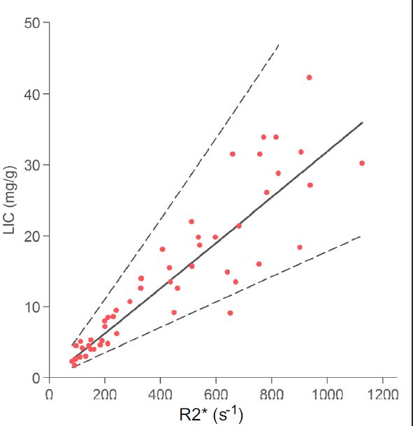
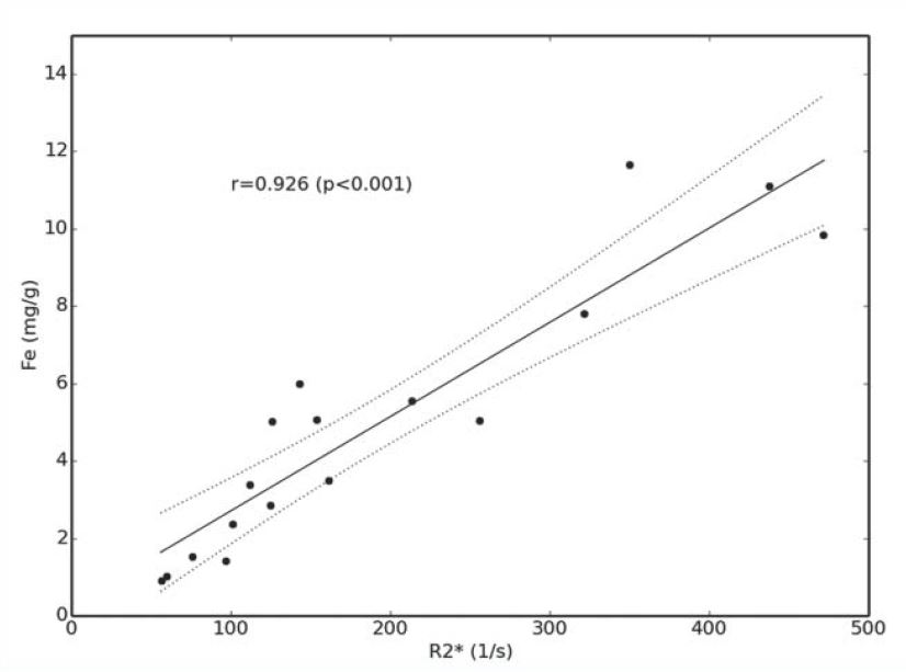
Graphically, here is the comparison of published correlations (R2* versus LIC expressed in mg/g, multiply by 18 to get μmol/g):
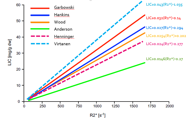
If you want a more complete comparison of the studies I advise you to read the article of Henninger.
It is necessary to redouble caution with maps calculated by dedicated 3D sequences because they make an estimate pixel by pixel and they become very heterogeneous in case of very high overload in iron, whatever the manufacturer of the MR system.
At 3 Tesla
So far only our study has been published:
| Ref | Patients | With biopsies | LIC range (mg/g) |
Sequence | Matrix | TR (ms) |
FA (°) |
TE-min (ms) |
delta-TE (ms) |
N TEs | TE-max (ms) |
Comment | Method | Correlation (R) |
|---|---|---|---|---|---|---|---|---|---|---|---|---|---|---|
| d'Assignies Eur Radiol 2018 |
105 patients | 105: hemochromatosis (n=31) DIOS (n=22) others (n=3) controls (n=49) |
0-35 | GRE multi echo |
106×128 | 120 | 20 | 1.2 | 1.2 | 10 | 12 | subtraction | 0.95 | |
| A total of 105 biopsies | ||||||||||||||
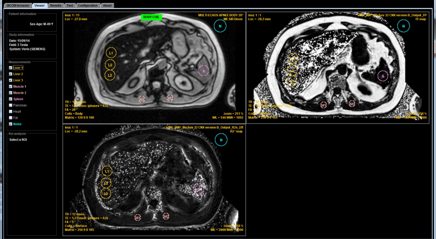
This study shows that, with a minimum TE of 1.2 ms, we can correctly calculate a T2* only for low or moderate overloads, less than 120μmol/g. One can not rely solely on the T2* result because higher overloads can be responsible for a significant underestimation of the iron concentration. It is therefore preferable to compare to the estimate obtained according to the SIR method and for that purpose to realize the sequence that we propose with the body antenna in order to be able to compare the signal between the liver and the muscles. If this sequence has not been obtained, do not rely on a result provided by a calculation of T2* (or R2*) if it is discordant with the observed signal. Even more than at 1.5T, maps calculated by dedicated 3D sequences become very heterogeneous and erroneous in case of major overload.
Whatever the magnetic field, a number of questions are not yet solved:
- How determine that a R2* map is wrong ? In some case it is easy if we have a look at the images (please do not fully delegate to a technician or a young resident without explaining him how to check the quality results) showing a noisy map with an elevated fat fraction. But in other case the value is just imprecise and you could have an underestimation. To solve it you need to have an access to the images from the different echoes. If there is a collapse of the liver signal on all the echoes including the first one you cannot trust the R2* value. The best is to double-check with a basic ME GRE sequence, preferably acquired with the body coil to have simultaneously SIR method.
- What differences do we obtain in practice with the various T2* calculation methods? The substraction method gives lower values but for the rest it is not necessarily easy to answer because it depends on several factors, the main ones are the presence of an associated steatosis or the importance of overload. It becomes even more complex to answer this question if we consider the maps produced by the specific 3D sequences proposed by the MRI vendors because the integrated calculation methods can be complex.
- And so what difference will be observed between two examinations performed in the same patient at 1.5 and 3T? This is not solved yet.
Advantages and disadvantages of both methods
| Method | Advantages | Disadvantages |
|---|---|---|
| SIR |
|
|
| R2* |
|
|
Quantification of the fat
In histology, in case of hepatic fat overload, lipid vacuoles appear in the cytoplasm of the hepatocytes. They are more or less numerous and of variable size. A semi-quantitative grade makes it possible to assess the percentage of hepatocytes that contain vacuoles. Thus, if all the hepatocytes contain at least one vacuole we get a grade of 100% but that does not mean that the hepatic fat concentration is 100%. If we want to obtain a fat fraction that can be compared with the fat quantification obtained by MRI, it is necessary either to analyze the biopsy fragment biochemically or to estimate, and it is simpler, the surface proportion of the cells. vacuoles in relation to the entire tissue. Few histomorphometry methods have been published and compared to biochemistry.
MRI uses the slight variation in resonant frequency of fat with respect to water to dissociate the two components and to quantify them.
several environments of the hydrogen atoms according to the bonds with the carbon atom.each environment is responsible for a small difference in frequency. Hamilton quantified the usual distribution of major components and their deviation in ppm from the peak of water.
| Composant | Proportion (%) |
delta/water (ppm) |
Frequency delta (hz) |
Phase cycle (ms) |
1.5T | 3T | 1.5T | 3T | ||||||
|---|---|---|---|---|---|---|---|---|---|---|---|---|---|---|
| 70 | -3.4 | -217 | -434 | 4.6 | 2.3 | |||||||||
| 12 | -2.6 | -166 | -332 | 6 | 3.0 | |||||||||
| 8.8 | -3.7 | -242 | -485 | 4.12 | 2.06 | |||||||||
| 4.7 | 0.7 | 38 | 77 | 26.3 | 13.1 | |||||||||
| 3.9 | -0.4 | -32 | -64 | 31.2 | 15.6 | |||||||||
| 0.6 | -2.75 | -125 | -249 | 2.0 | 4.01 | |||||||||
| Practically, we observed a phase cycle of 4.8ms at 1.5T and of 2.4 ms at 3T. | ||||||||||||||
There are therefore two main methods for quantifying hepatic steatosis (and, more generally, any microscopic fat infiltration): either spectroscopy in a small volume, or phase imaging by studying the variation of the signal (and / or phase) with from images obtained by multiple TEs. Of course this acquisition should preferably be a single sequence with multiple echoes, as for the calculation of T2*.
MRI spectroscopy or spectroMR
The spectroMR technique is theoretically the most efficient for exact quantification of steatosis. It was validated against the biopsy, comparing most often with the grade. It would be particularly interesting if we could analyze the variations of proportion of the different components but in practice the acquisition remains difficult imposing a good compensation of the homogeneity of the magnetic field (shim). It often lacks robustness, especially in case of presence of hepatic iron overload even if it is not very marked. Apnea acquisition is now possible but the information quality is limited compared to what can be achieved for other motionless organs.
Also the use of spectroMR is not a daily practice for quantification of steatosis. This is especially true since the simpler methods to implement and based on phase imaging have been proposed.
Phase Imaging
It is based on the use of gradient echo sequences comprising TEs :
- in-phase (multiples of 4.8ms to 1.5T and 2.4ms to 3T) with the signal of fat and liver tissue (water) that add up,
- and opposed-phase with the signal of fat that is subtracted from the hepatic signal. The first TE in opposed-phase is, at 1.5T, 2.4ms and the following are spaced 4.8ms or 7.2ms, 12ms etc, and at 3T of 2.4ms and the following spaced 2.4ms that is 3.6ms; 6ms etc.
Thus the signal difference between the 2 acquisitions in phase and in opposed-phase corresponds to the signal of the fat. The formula of DIXON using these two points is simple:
When there is as much of fat than liver (FF = 50%) a complete cancellation of the signal is obtained. Beyond that, which is really exceptional for a liver of steatosis, we have a rise of the signal and at the maximum, for pure fat, the signal is even superior to that of a non-steatotic liver, especially if there is still a T1-weighting. A result of 25% FF would be comparable to that of a 75% FF. In practice, this ambiguity is not a problem for the quantification of hepatic fat because a steatosis with a FF of 50% is practically a maximum. An exceptional FF of 55% will be confused with a FF of 45%. In all cases the histological grade would have been 100%.
But before using this signal difference, the effect of other factors must be reduced:
- the T2* effect responsible for the progressive decline of the signal with the increase of the TE. In the absence of steatosis there could be a slight negative value which increases when there is an iron overload. The calculation of Dixon 2 points is therefore interesting in practice for the diagnosis of these two pathologies ... as long as they are not associated because otherwise the two modifications are opposed. The T2* effect can be reduced:
- either by using the signal average of the first two in-phase TE and comparing it to the opposed-phase TE that is in between. This is called the Dixon 3 points method:
in-phase 1 = opposed-phase 2 = and in-phase 2 = => fat fraction = %
- either by calculating the T2* from the points in phase and the T2* from the points in opposition of phase and by measuring the proportional difference between the two curves.
- either by using the signal average of the first two in-phase TE and comparing it to the opposed-phase TE that is in between. This is called the Dixon 3 points method:
- the T1 effect because the fat has a very short T1 and its signal is much higher than that of the liver in T1-weighted sequence. It is therefore limited by reducing the T1-weighting by a low flip angle. It must be reduced according to the TR used. For example, an angle of 20° with a TR of 120 ms is acceptable but it is necessary to go down to an angle of 3 or 4 ° if the TR is less than 30 ms.
- the different components of the fat do not have the same phase shift and complete signal modeling can be done by including several fat components or "peaks". This is called multipeak modeling.
- T2 of fat is also longer than T2 of liver and this can complicate the model.
Currently all manufacturers provide multi-echo 3D sequences that produce maps of fat fraction trying to manage, with more or less success, the ambiguity between 0 and 100%. Quantification method is based on slightly different principles. It is efficient as long as there is not too much iron overload.
We can also use the quantification software MRQuantif which is using data from a standardized multi echo 2D sequence, available on all devices, to quantify steatosis and iron overload in a single time, to write an automatic report and to archive this data. The software integrates the different calculation methods and is configurable. It takes into account the level of iron overload to accept or reject the estimate obtained from the MRI signal.