Warning: include(/data/htdocs/hebergementweb/sites/imagemed.univ-rennes1.fr/en/nav.html): failed to open stream: No such file or directory in /data/htdocs/hebergementweb/sites/imagemed.univ-rennes1.fr/template.php on line 144
Warning: include(): Failed opening '/data/htdocs/hebergementweb/sites/imagemed.univ-rennes1.fr/en/nav.html' for inclusion (include_path='.:/usr/share/pear:/data/htdocs/hebergementweb/php-include') in /data/htdocs/hebergementweb/sites/imagemed.univ-rennes1.fr/template.php on line 144
MRQuantif 'Results': curve and concentrations
This screen displays, if possible, a graph representing the decay curves of the signal. In the left panel you can select parameters influencing the results displayed in this section but also in the following textsection. These are mostly the selected series (if multiple series are available), the conversion unit for iron concentration, and calculation methods. In parallel the report is copied to the clipboard of the computer ready to be pasted into a report of the RIS software according to the defined parameters.
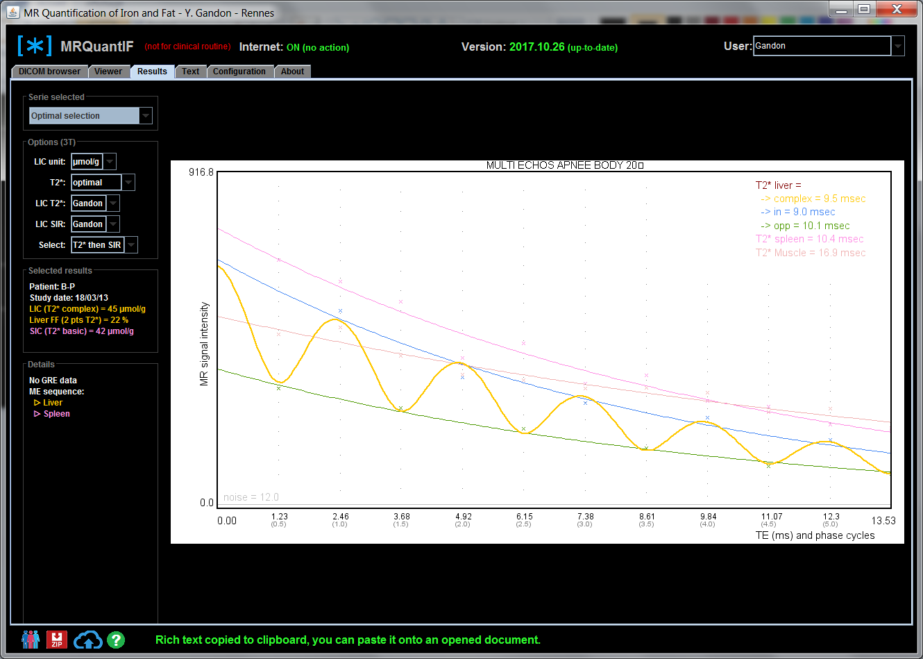
The central chart
This area potentially displays a graph if at least one multi-echo sequence has been selected. It shows the decay of the MRI signal as a function of the echo time (TE) expressed in milliseconds but also, in parentheses) in the number of phases.
There is, according to the available information:
- the measured points of the signal of the liver, muscle, spleen ... at the different values of the echo times. For the liver, the color of the dots changes to blue, green or black depending on whether they are considered, respectively, as close to the phase, phase opposition or intermediate.
- an orange curve of calculated decay of the hepatic signal:
- or preferably using the complex signal information, if at least one peak (3 by default) has been chosen in the configurationsection. It therefore ripples in case of steatosis.
- using the value of T2 * basiccalculated from all liver points.
- a blue curve of decay of the hepatic signal according to the T2 * incalculated from the in-phase points.
- a green curve of decay of the hepatic signal according to the T2 * outcalculated from the in-phase points.
- a light brown curve of decay of the muscular signal according to the T2 * basiccalculated from all muscle points.
- a purple splenic signal decay curve according to the T2 * basiccalculated from all splenic points.
- the T2 * values obtained in the upper right corner.
- and at the bottom of the graph, the basic gray line of the background noise with the average value of the signal measured by all the corresponding ROIs or the calculation of the offset via the calculation of the T2 * offset .
The right panel
The selection of the series
If several multi-echo sequences are selected the software determines the optimal sequence taking into account the acquisition parameters. It will preferably choose a sequence with a TR close to 120 ms, a FA close to 20 °, multiple TEs if possible of 1.2 ms, an antenna Body... The different sequences (including the sequence considered optimal) can be chosen from a drop-down menu.
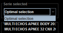
The choice of a series modifies the curve but also the values of the results and potentially the report.
The options
This is a very important part of the software. The different options available influence the value of the results:
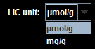
- LIC unit: You can choose to use the unit of expression of hepatic iron concentration per gram of liver (dry weight) by selecting either μmol/g if you work with hepatologists or mg/g if you work with hematologists. There is a factor 18 between these two values: 1 mg/g = 18 μmol/g. This explains why the upper limit of the normal initially fixed at 2 mg/g is also 36 μmol/g.
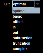
- T2 *: the software proposes different methods of calculation of T2 * (only for the liver):
- T2 * optimal: the software chosen T2 * that seems optimal taking into account the values obtained and the correlation coefficient at the points used.
- T2 * basic: this is the calculation of the T2 * taking all the points of the liver, without taking into account the phase and without taking into account any background noise measured or calculated . It is understood that the measurement can be disturbed by the presence of fat or distorted in the event of significant collapse of the signal.
- T2 * offset: it's the same thing but considering that there is an offset corresponding to the background noise. This unknown is calculated by the formula. In practice, the offset value obtained is sometimes false and far from the measured value of the background noise.
- T2 * in: this is the calculation of the T2 * basic but taking only the points of the liver close to the phase.
- T2 * out: this is the calculation of the T2 * basic but taking only the points of the liver close to the phase opposition.
- T2 * subtraction: it's the same as the T2 * basic, but subtracting the background signal from the liver signal (calculated by offset or measured). This method often leads to a reduction in T2 *.
- T2 * truncation: it's the same as the T2 * basic but stopping to take into account the points of the hepatic signal from the first point which is equal to or less than background noise. It is certainly the most logical method but it can also be faulted if the signal is collapsed.
- T2 * extrapolation: it's the same as the T2 * truncation but adding fictitious points adapted to the shape of the curve (personal idea not yet evaluated).
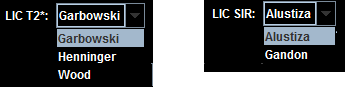
- LIC T2 *: the software allows you to choose the conversion formula that gives the hepatic iron concentration (CHF or LIC in English) from T2 * or R2 * (T2 * = 1/R2 * and vice versa). At 1.5T, there are several published references giving slightly different results (Garbowski 2014, Henninger and Wood). If you work with a formula you can select it, otherwise by default and in a recommended way for now choose instead that of Garbowski. At 3T, there is only one reference.
- LIC SIR: the software also allows you to choose the algorithm for calculating the hepatic iron concentration (CHF or LIC in English) from the liver-to-muscle ratio. At 1.5T, there are two published references giving different results (Alustiza and Gandon). If you work with a formula you can select it, otherwise by default and in a recommended way for now choose instead of Alustiza. Indeed the method we propose probably increases the average iron overload. At 3T, there is only, up to know, one reference.
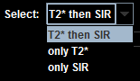
- Select: finally it is possible to define if one wishes to prioritize one of the two methods, T2 * or SIR, or if the system has to take into account the T2 * in priority and to use the SIR method if the measured T2 * is too short compared to the shortest TE used (T2 * <2 TE min) or if the correlation between the T2 * curve and the measured signal is not high enough (r2 <0.8).
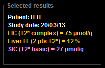
The selected results
In the underlying area the selected results give liver iron concentration (LIC), hepatic fatty fraction (FF) and also splenic iron concentration (LIC) or other organ results if an ROI has been awarded.
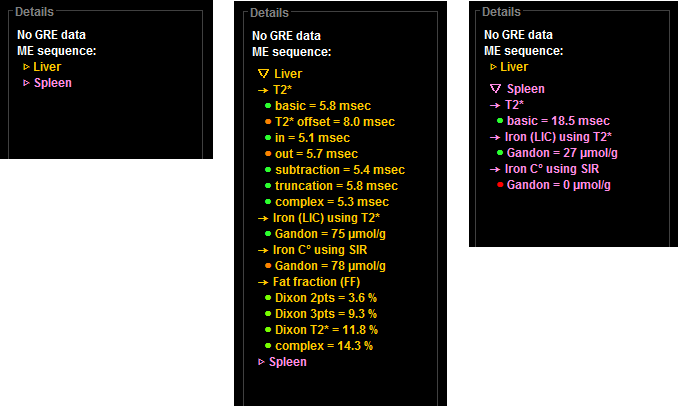
The detailed results
Finally it is possible to consult the detailed results by organ by opening the corresponding block. Before each value is placed a chip of color:  green if the result is admissible,
  orange s' it is more uncertain or
  red if it is probably wrong or if the method is not suitable.
The decisions of an international working group that will meet in March 2018 or future published results may change default preferences in future releases.